Langevin-based method estimates resilience of non-stationary systems without heavy data pre-processing
Authors report a regression-based Langevin method that handles seasonality, irregular sampling and data gaps, tested on synthetic series and real vegetation, paleoclimate and glacier data.
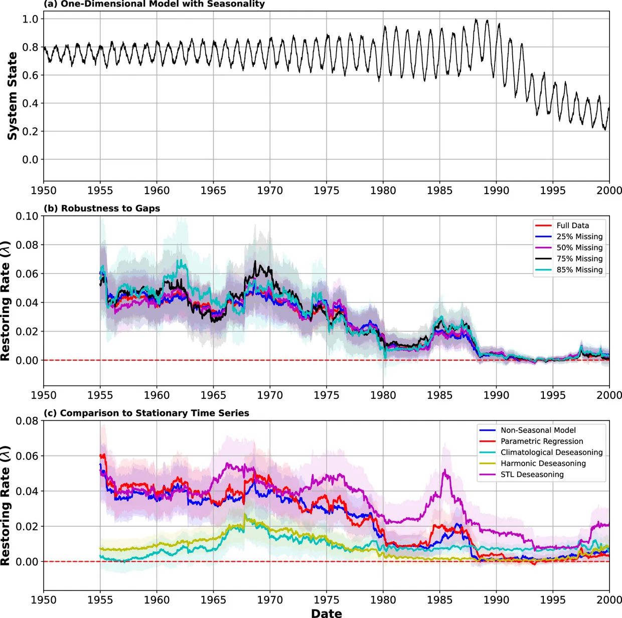
A paper in Nature Communications introduces a method for estimating the resilience of systems whose dynamics are not stationary, such as global vegetation under strong seasonal forcing. The authors quantify resilience as a recovery rate λ and estimate it directly with a regression-based formulation of the Langevin equation. They tested the method on synthetic time series and on real-world data: vegetation dynamics, paleoclimate proxies and glacier surges. nature.com
Nature Communicationsnature.comOpen source ↗
According to the authors, the method needs no extensive data pre-processing, tolerates gaps in the record and does not require regular time sampling. It can include time-varying data uncertainties, give uncertainty bounds for stability estimates and extend to spatial systems. The authors call it a drop-in replacement for widely used autocorrelation-based resilience estimates.
Limits of critical slowing down metrics
Many studies estimate the stability of Earth system components through critical slowing down, where system dynamics slow as a critical transition approaches. Lag-1 autocorrelation (AC1) and variance are the most common early warning indicators. Most such metrics rely on evenly sampled time series and on stationarity, meaning no trend and no seasonality within the analysis window.
Even sampling is not guaranteed, for example in paleoclimate proxy records or in composites of several datasets. Stationarity is usually achieved by deseasoning and detrending, which the authors describe as error-prone. Changes in sensor signal-to-noise ratio, unrelated to loss of stability, can also shift AC1 and variance, and current methods struggle to include data uncertainty. nature.com
Nature Communicationsnature.comOpen source ↗
How the regression approach works
The system state is treated as a stochastic Markov process around a time-dependent attractor that can be fixed, drifting or oscillating. Near the attractor, the restoring force is approximated as linear, and its gradient is λ; a decrease of λ toward zero signals loss of resilience.
Instead of removing the attractor's movement by detrending, the method takes its functional form as a starting point. The change in system state is split into a part that depends linearly on the state and a part that comes from external forcing and is a function of time. λ is estimated in moving temporal windows, within which resilience and noise strength are assumed constant; the window size must match the speed of the system dynamics. External perturbations, such as rainfall over a region, are assumed homogeneous, so spatial variation is attributed to noise and internal feedbacks.